
Real sensor beam tables
A spinning LiDAR is not a fan of evenly spaced beams. A VLP-32C puts seventeen of its thirty-two lasers inside a 0.333 degree band around the horizon and spends 9.36 degrees on the gap below it, because the objects a car needs to see are near the horizon. How many rings land on a pedestrian at forty metres is decided by that table and by nothing else, so a simulator that can only interpolate between a minimum and a maximum elevation cannot reproduce any real sensor.
- Sensors
- 7 named heads, Velodyne and Ouster
- Tables
- Elevations in firing order, from vendor calibration files
- Per point
- x y z, intensity, ring, instance, class, time in microseconds
- Provenance
- Derived values named in capture.json
The difference a table makes
Both captures below are the same scene, the same seed, the same thirty-two channels and the same vertical field from minus 25 to plus 15 degrees. The only difference is the table. On the left, the VLP-32C’s measured elevations; on the right, the even ladder every open-source simulator produces when you give it those two numbers.
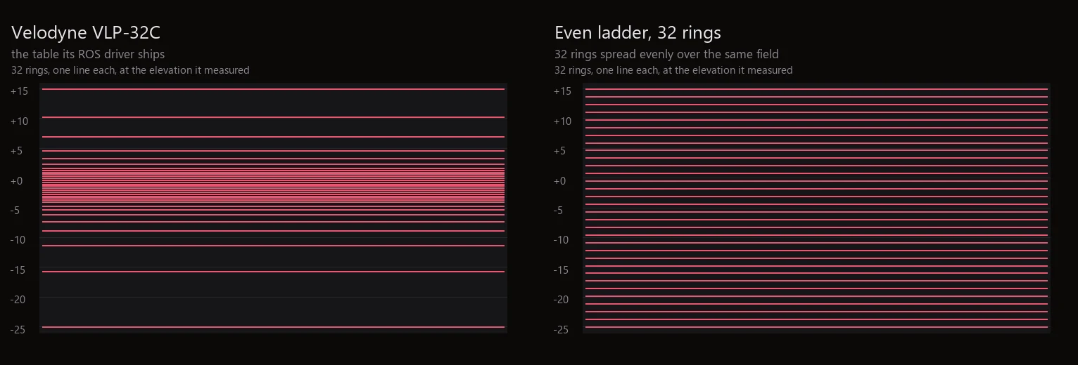
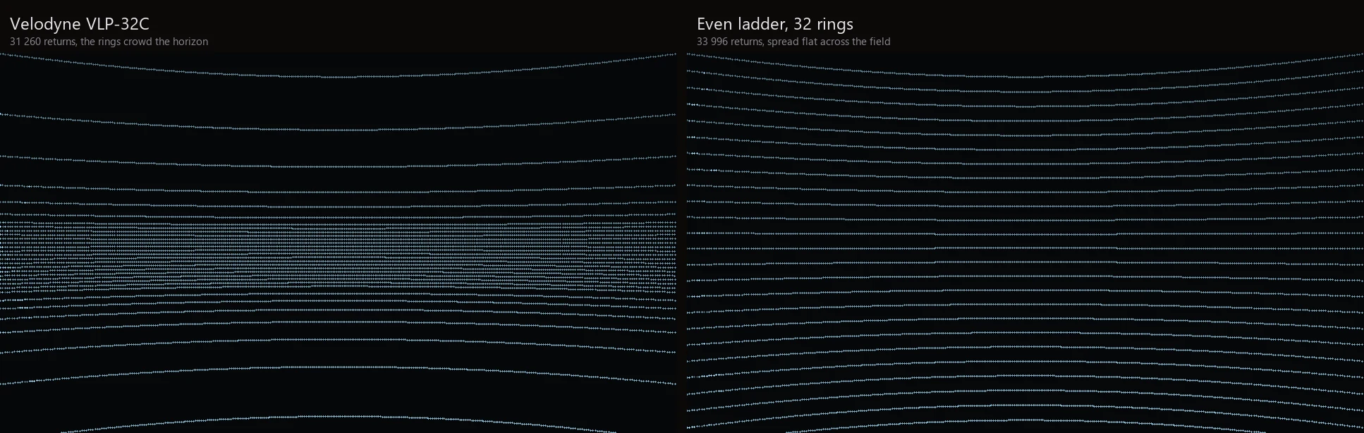
Same channel count, same field, different sensor. A detector trained on the right cloud has learned a ring spacing no hardware produces, and finds out on the day it meets the real one.
The sensors
| Sensor | Channels | Vertical field | Character |
|---|---|---|---|
| Velodyne VLP-16 Puck | 16 | -15° to +15° | Uniform 2.0° spacing, the entry-level head |
| Velodyne HDL-32E | 32 | -30.67° to +10.67° | Uniform 1.33°, biased downward |
| Velodyne VLP-32C Ultra Puck | 32 | -25° to +15° | Strongly non-uniform: 0.333° near the horizon, 9.36° at the bottom |
| Velodyne HDL-64E S3 | 64 | -24.71° to +2.02° | Two blocks, dense above the horizon. The KITTI sensor |
| Ouster OS1-64 | 64 | -21.2° to +21.2° | Ouster's Uniform beam layout, 200 m range |
| Ouster OS1-128 | 128 | -21.2° to +21.2° | The dense long-range head |
| Ouster OS0-128 | 128 | -45° to +45° | A 90 degree field for close range around a robot |
The elevations come from the calibration files the vendors’ ROS drivers ship, in firing order rather than sorted, because firing order is what per-point timing depends on. Where a value is derived rather than published, the profile says so and the derivation is written into capture.json under lidar.beams.approximations. The HDL-64E is the clearest case: its two laser blocks have published endpoints but no published per-laser angles, so the record says the angles inside each block are spread evenly, rather than leaving a reader to assume a calibration file behind them. A dataset built on a derived table cannot be mistaken for one built on a measured one.
Choosing a sensor in the Studio hides the channel count and vertical field controls, because those two numbers are consequences of the table rather than settings. Rotation rate, points per turn, range and both noise figures stay editable, because they are configurable on the hardware too. A custom mode keeps the plain two-number field for a head that is not in the list.
Every point knows when it was fired
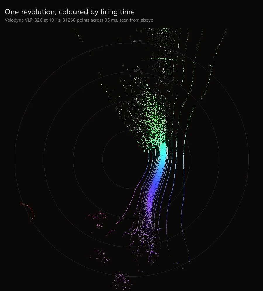
A real head does not photograph a scene, it sweeps one. A revolution at 10 Hz takes a tenth of a second, and each laser fires at its own offset inside the firing cycle. Every point NameFrame writes carries that time: the column’s fraction of the revolution plus the laser’s own offset, in microseconds, as a time_us column in the PLY and as lidar.times.bin beside the KITTI file, whose four-float record has no room for it. Anything doing odometry or de-skewing needs those times, and a sweep that reports one timestamp for every point quietly tells it the vehicle never moved.
Motion within the sweep
A vehicle carrying a spinning head does not wait for the revolution to finish, so the returns at the end of a sweep are taken from somewhere else than the returns at the start. That mismatch is what de-skewing exists to undo, and a simulator that samples the whole cloud from one pose quietly deletes it from the data.
With motion enabled, each ray leaves from where the sensor has reached by its own firing time, and the return is still written against the pose the frame publishes: exactly the skew a real cloud carries. The velocity comes from the previous frame at the declared frame rate, and lidar.json records it in the point convention, so a consumer can undo the skew with the numbers as written.
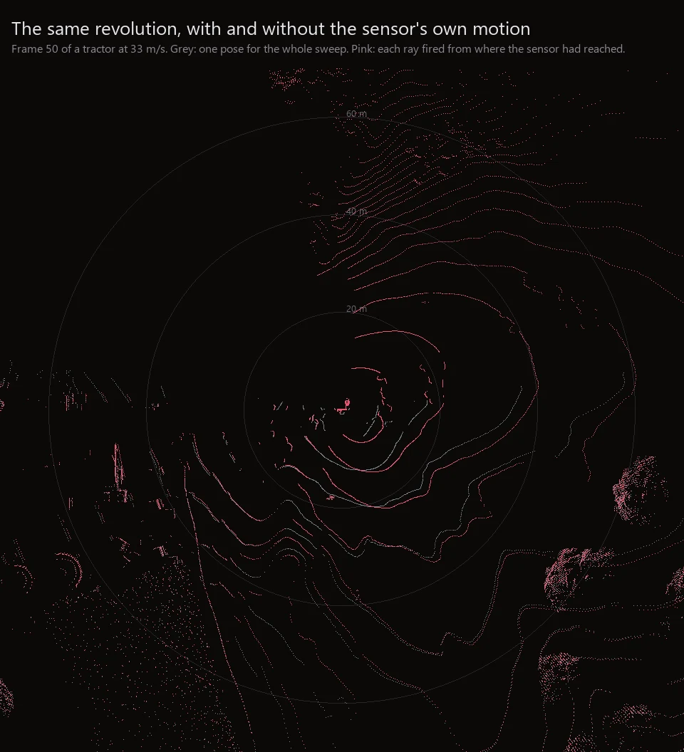
Measured against the matched still capture with the noise zeroed: rays fired in the first millisecond of the revolution moved 0.018 m where velocity times time predicts 0.017, growing to about three metres by the end of the turn. It is off unless asked for, it requires a video capture because that is what defines the interval a velocity is measured over, and where it cannot be measured, the first frame of a run, or a camera cut, the frame records the refusal and the reason instead of quietly writing an unskewed sweep.
What no other Unreal Engine tool writes per point
| Field | Where it lives | What it is for |
|---|---|---|
| x, y, z | lidar.ply, lidar.bin | KITTI convention, metres |
| intensity | lidar.ply, lidar.bin | Incidence and range falloff, with its own noise |
| ring | lidar.ply | Which laser produced the return |
| time_us | lidar.ply, lidar.times.bin | Microseconds from the start of the revolution |
| instance id, class id | lidar.labels.bin | The same numeric ids as the image mask of the same frame, so a fusion model can be evaluated across modalities |
The instance ids are the point. The boat that is instance 7 in the RGB mask is instance 7 in the point cloud, from the same frame, so image and cloud agree about which object is which without an annotation pass. An optional gate refuses a frame when an object visible in the image received no return at all, which is the failure that ruins a fusion dataset silently.